Parametric equations are presented with examples and their solutions. More questions with solutions are included.
\( \) \( \) \( \)
Examples
Example 1
Some curves are best described using parametric equations \( x \) and \( y \) in term of a parameter [1] [2] .
The following is an example of parametric equations \( x(t) \) and \( y(t) \) in term of the parameter \( t \).
\[
\begin{equation}
\left\{ \begin{aligned}
x(t) &= t \\\\
y(t) &= 0. 5 t^2 \qquad \text{for} t \in [0,3]
\end{aligned} \right.
\end{equation}
\]
The plot of the curve of the parametric equations is made by finding the \( x \) and \( y \) coordinates for different values of the parameter \( t \) as shown in the table below.
Table.1 Table of Values of The Parametric Equations \( x(t) = t \) and \( y(t) = 0. 5 t^2 \)
The plot of the curve defined by the parametric equations \( x(t) = t \) and \( y(t) = 0.5 t^2 \) for \( t \) in the range \( [0 , 3] \) is shown below.
Each values of \( t \) determine a point \( (x,y) \) which is plotted in a system of coordinates. As \( t \) varies, the
point \( (x(t), y(t)) \) traces out a curve called parametric curve .
The red arrows gives the direction of increase of the parameter \( t \).
Fig.1 Plot of the Curve Parametric Equations \( x(t) = t \) and \( y(t) = 0.5 t^2 \) Note that the curve obtained is part of a parabola that may be obtained by eliminating \( t \) as follows
Solve the first parametric equation \( x(t) = t \) for \( t \) to obtain.
\[ t = x \]
Substitute \( t \) by \( x \) in the second equation \( y(t) = 0.5 t^2 \) to obtain
\[ y = 0.5 x^2 \]
which is a parabola.
When taking the values of \( t \) in the range \( [0 , 3] \) only part of this parabola is shown.
Example 2
This example shows the advantage of using simple parametric equations to describe complex curves. The parametric equations given below describe the Lissajous curves used in Electrical engineering.
Let
\[
\begin{equation}
\left\{ \begin{aligned}
x(t) &= \sin t + 1 \\\\
y(t) &= \sin 2t + 2 \qquad \text{for} t \in [0,2\pi]
\end{aligned} \right.
\end{equation}
\]
The table of values of \( x \) and \( y \) for different values of the parameter \( t \), is shown below.
Table.2 Table of Values of The Parametric Equations \( x(t) = \sin t + 1 \) and \( y(t) = \sin 2t + 2\)
The plot of the curve defined by the parametric equations \( x(t) = \sin t + 1 \) and \( y(t) = \sin 2t + 2\) for \( t \) in the range \( [0 , 2\pi] \) is shown below with the arrows showing the direction of increase of the
parameter \( t \). This curve is one of
Fig.2 Plot of the Curve Parametric Equations \( x(t) = \sin t + 1 \) and \( y(t) = \sin 2t + 2 \)
Let us now find an equation of the curve in rectangular coordinates by elimination the parameter \( t \).
The first equation may be rewritten as
\[ \sin t = x - 1\]
Use the trigonometric identity \( \sin (2 t) = 2 \sin t \cos t \) to rewrite the second equation as
\[ y = 2 \sin t \cos t + 2 \]
Use the trigonometric identity \( \cos (t) = \pm \sqrt {1-\sin^2 t}\) to rewrite the above equation as
\[ y = \pm 2 \sin t \sqrt {1-\sin^2 t} + 2 \]
Substitute \( \sin t \) by \( x - 1 \) in the above equation to obtain
\[ y = \pm 2 (x - 1) \sqrt{1 - (x-1)^2} + 2 \]
Which may be written as
\[ y - 2 = \pm 2 (x - 1) \sqrt{1 - (x-1)^2} \]
Square both sides, simplify and write as one equation
\[ \left(y-2\right)^{2}=4\left(x-1\right)^{2}\left(2x-x^{2}\right) \]
Note that this example shows the simplicity of parametric equations in representing complex curves that may not be simple to describe by an equation in rectangular coordinates as shown above.
Questions
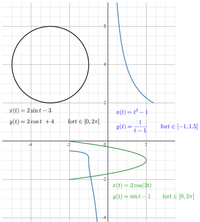
Find an equation in rectangular coordinates to describe the curve whose parametric equations are given below and then plot the curves of all three sets of parametric equations.
Solve the equation \( x = t^3 - 1 \) for \( t \)
\[ t = \sqrt[3]{x + 1} \]
Substitute \( t \) by \( \sqrt[3]{x + 1} \) in \( y \)
\[ \boxed { y = \dfrac{1}{\sqrt[3]{x + 1}-1} } \]
Rewrite the equation \( x = 2 \sin t - 3 \) as
\[ \sin t = \dfrac{x+3}{2} \]
Rewrite the equation \( y = 2 \cos t + 4 \) as
\[ \cos t = \dfrac{t - 4}{2} \]
Substitute \( \sin t \) and \( \cos t \) in the trigonometric identity \( \sin^2 t + \cos^2 t = 1 \) by their expressions to write
\[ \left(\dfrac{x+3}{2}\right)^2 + \left(\dfrac{t - 4}{2}\right)^2 = 1 \]
Simplify and rewrite as
\[ \boxed { (x+3)^2 + (y-4)^2 = 2^2 } \]
Note that the above is the equation of a circle with center at \( (-3,4) \) and radius euql to \( 2 \)
Use the trigonometric identity \( \cos (2t) = 1 - 2 \sin^2 t \) to rewrite the equation \( x = 2 \cos (2 t) \) as
\[ x = 2 (1-2 \sin^2 t) \]
Rewrite the equation \( y = \sin t - 1 \) as
\[ \sin t = y + 1 \]
Substitute \( \sin t \) in \( x = 2 (1-2 \sin^2 t) \) by \( y + 1 \) to obtain
\[ \boxed { x = 2-4(y+1)^2 } \]
Note that the above is the equation of a parabola with horizontal axis and vertex at \( (2,-1) \)
Fig.3 Plot of the Curves of All Parametric Equations Given Above
More References
University Calculus - Early Transcendental - Joel Hass, Maurice D. Weir, George B. Thomas, Jr., Christopher Heil - ISBN-13 : 978-0134995540
Calculus - Early Transcendental - James Stewart - ISBN-13: 978-0-495-01166-8