Matrices Applied to Electric Circuits

This tutorial demonstrates how mathematics, specifically matrices and linear systems, can be applied to model and solve complex electric circuits using Kirchhoff's laws.

Circuit Modeling with Kirchhoff's Laws

Consider the electric circuit illustrated below, containing two closed loops: Loop 1 (\(e_1, R_1, R_3\)) and Loop 2 (\(e_2, R_2, R_3\)). Here, \(e_1\) and \(e_2\) are voltage sources, \(R_1, R_2, R_3\) are resistors, \(i_1\) is the current flowing across \(R_1\), and \(i_2\) is the current flowing across \(R_2\).
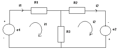
electric circuit diagram

Applying Kirchhoff's Voltage Law to each loop gives:

The Problem: If the voltage sources (\(e_1, e_2\)) and resistances (\(R_1, R_2, R_3\)) are known, how do we calculate currents \(i_1\) and \(i_2\)? While this two-loop circuit is simple, larger networks involve many more equations, making matrix representation essential.

Matrix Form of the Circuit Equations

First, group like terms in the system of equations:

We can then write this system in matrix form: \[ \begin{bmatrix} e1 \\ e2 \end{bmatrix} = \begin{bmatrix} R1+R3 & -R3 \\ -R3 & R2+R3 \end{bmatrix} \begin{bmatrix} i1 \\ i2 \end{bmatrix} \] Let matrices \(e\), \(R\), and \(i\) be defined as: \[ e = \begin{bmatrix} e1 \\ e2 \end{bmatrix} \quad , \quad R = \begin{bmatrix} R1+R3 & -R3 \\ -R3 & R2+R3 \end{bmatrix} \quad , \quad i = \begin{bmatrix} i1 \\ i2 \end{bmatrix} \] and write the system of equations using matrices as follows \[ e = R i \] The solution to the above matrix equation is given by: \[ i = R^{-1}e \] where \(R^{-1}\) is the inverse of the resistance matrix \(R\), computed as: \[ R^{-1} = \frac{1}{(R1+R3)(R2+R3)-(R3)^2} \begin{bmatrix} R2+R3 & R3 \\ R3 & R1+R3 \end{bmatrix} \]

More Resources


Home Page