El problema de mínimos cuadrados es encontrar una solución aproximada
Se muestra en Álgebra Lineal y sus Aplicaciones que la solución aproximada
En muchas aplicaciones de la vida real, cuando no se puede encontrar una solución x para un sistema de ecuaciones de la forma
A x = B
(el sistema es inconsistente), es posible que una solución aproximada ![]() para el sistema dado A x = B sea suficiente.
para el sistema dado A x = B sea suficiente.
El problema de mínimos cuadrados es encontrar una solución aproximada ![]() tal que la distancia entre los vectores A x y B dada por
tal que la distancia entre los vectores A x y B dada por ![]() sea la más pequeña.
sea la más pequeña.
Se muestra en Álgebra Lineal y sus Aplicaciones que la solución aproximada ![]() está dada por la ecuación normal
está dada por la ecuación normal
![]() donde AT es la transpuesta de la matriz A .
donde AT es la transpuesta de la matriz A .
Ejemplo 1
a) Demuestre que el sistema A x = B con
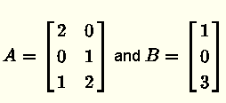 es inconsistente (sistema sin soluciones).
b) Encuentre la solución de mínimos cuadrados para el sistema inconsistente A x = B .
c) Determine el error de mínimos cuadrados dado por || A \hat x - B || para la solución encontrada en la parte b).
Solución del Ejemplo 1
a)
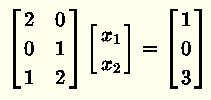
El sistema de ecuaciones a resolver se puede escribir en la forma
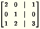
Escriba el sistema anterior en forma de matriz aumentada
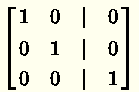
Reduzca por filas (Gauss-Jordan) la matriz aumentada anterior
 \( \) \( \) \( \) \( \)
La última fila da la ecuación \( 0 \cdot x_1 + 0 \cdot x_2 = 1 \) que no tiene solución y por lo tanto el sistema es inconsistente.
b)
Encontremos \( A^T \)
\( A^T =
\begin{bmatrix}
2 & 0 & 1\\
0 & 1 & 2
\end{bmatrix}
\)
Calcule \( A^T A \) y \( A^T B \)
\( A^T A =
\begin{bmatrix}
2 & 0 & 1\\
0 & 1 & 2
\end{bmatrix} \cdot
\begin{bmatrix}
2 & 0 \\
0 & 1 \\
1 & 2
\end{bmatrix} =
\begin{bmatrix}
5 & 2\\
2 & 5
\end{bmatrix}
\)
\( A^T B =
\begin{bmatrix}
2 & 0 & 1\\
0 & 1 & 2
\end{bmatrix} \cdot
\begin{bmatrix}
1 \\
0 \\
3
\end{bmatrix} =
\begin{bmatrix}
5\\
6
\end{bmatrix}
\)
Sustituya \( A^T A \) y \( A^T B \) por sus valores numéricos en la ecuación normal \( A^T A \hat x = A^T B \), obtenemos el sistema
\(
\begin{bmatrix}
5 & 2\\
2 & 5
\end{bmatrix}
\cdot \hat x =
\begin{bmatrix}
5\\
6
\end{bmatrix}
\)
Resuelva lo anterior para obtener
\( \hat x =
\begin{bmatrix}
\dfrac{13}{21}\\
\dfrac{20}{21}
\end{bmatrix}
\)
c)
\( A \cdot \hat x - B =
\begin{bmatrix}
2 & 0 \\
0 & 1 \\
1 & 2
\end{bmatrix}
\begin{bmatrix}
\dfrac{13}{21}\\
\dfrac{20}{21}
\end{bmatrix} -
\begin{bmatrix}
1 \\
0 \\
3
\end{bmatrix} =
\begin{bmatrix}
\dfrac{5}{21}\\
\dfrac{20}{21}\\
- \dfrac{10}{21}
\end{bmatrix}
\)
\( || A \cdot \hat x - B || = \sqrt { \left(\dfrac{5}{21}\right)^2 + \left(\dfrac{20}{21}\right)^2 + \left(- \dfrac{10}{21}\right)^2 } = \dfrac{5\sqrt{21}}{21} \approx 1.1 \)
Ejemplo 2
a) Demuestre que el sistema \( A x = B \) con
\( A =
\begin{bmatrix}
1 & 0 & 1\\
2 & 0 & 2 \\
0 & -1 & 1\\
0 & -2 & 2
\end{bmatrix}
\) y \( B =
\begin{bmatrix}
2 \\
3 \\
4 \\
7
\end{bmatrix}
\)
es inconsistente.
b) Encuentre la solución de mínimos cuadrados para el sistema inconsistente \( A x = B \).
c) Determine el error de mínimos cuadrados dado por \( || Ax - B || \) para la solución encontrada en la parte b).
Solución del Ejemplo 2
a)
El sistema de ecuaciones a resolver se puede escribir en la forma
\[
\begin{bmatrix}
1 & 0 & 1\\
2 & 0 & 2 \\
0 & -1 & 1\\
0 & -2 & 2
\end{bmatrix}
\begin{bmatrix}
x_1\\
x_2 \\
x_3
\end{bmatrix}
=
\begin{bmatrix}
2 \\
3 \\
4 \\
7
\end{bmatrix}
\]
Escriba el sistema anterior en forma de matriz aumentada
\(
\begin{bmatrix}
1 & 0 & 1 & |& 2\\
2 & 0 & 2 & | & 3 \\
0 & -1 & 1 & | & 4 \\
0 & -2 & 2 & | & 7
\end{bmatrix}
\)
Escriba en forma reducida por filas (Gauss-Jordan)
\(
\begin{bmatrix}
1 & 0 & 1 & | & 0\\
0 & 1 & -1 & | & 0 \\
0 & 0 & 0 & | & 1 \\
0 & 0 & 0 & | & 0
\end{bmatrix}
\)
La tercera fila da la ecuación \( 0 \cdot x_1 + 0 \cdot x_2 + 0 \cdot x_3 = 1 \) que no tiene solución y por lo tanto el sistema es inconsistente.
b)
Primero encontremos \( A^T \)
\( A^T =
\begin{bmatrix}
1 & 2 & 0 & 0\\
0 & 0 & -1 & -2\\
1 & 2 & 1 & 2
\end{bmatrix}
\)
Calcule \( A^T A \) y \( A^T B \)
\( A^T A =
\begin{bmatrix}
1 & 2 & 0 & 0\\
0 & 0 & -1 & -2\\
1 & 2 & 1 & 2
\end{bmatrix} \cdot
\begin{bmatrix}
1 & 0 & 1\\
2 & 0 & 2 \\
0 & -1 & 1\\
0 & -2 & 2
\end{bmatrix} =
\begin{bmatrix}
5 & 0 & 5\\
0 & 5 & -5\\
5 & -5 & 10
\end{bmatrix}
\)
\( A^T B =
\begin{bmatrix}
1 & 2 & 0 & 0\\
0 & 0 & -1 & -2\\
1 & 2 & 1 & 2
\end{bmatrix} \cdot
\begin{bmatrix}
2 \\
3 \\
4 \\
7
\end{bmatrix} =
\begin{bmatrix}
8\\
-18\\
26
\end{bmatrix}
\)
Sustituya \( A^T A \) y \( A^T B \) por sus valores numéricos en la ecuación normal \( A^T A \hat x = A^T B \), obtenemos el sistema
\(
\begin{bmatrix}
5 & 0 & 5\\
0 & 5 & -5\\
5 & -5 & 10
\end{bmatrix}
\cdot \hat x =
\begin{bmatrix}
8\\
-18\\
26
\end{bmatrix}
\)
Escriba el sistema anterior en forma de matriz aumentada
\(
\begin{bmatrix}
5 & 0 & 5 & | & 8\\
0 & 5 & -5 & | & -18\\
5 & -5 & 10 & | & 26
\end{bmatrix}
\)
Reduzca por filas la matriz anterior
\(
\begin{bmatrix}
1 & 0 & 1 & | & \dfrac{8}{5}\\
0 & 1 & -1 & | & -\dfrac{18}{5}\\
0 & 0 & 0 & | & 0
\end{bmatrix}
\)
\( x_3 \) es la variable libre.
segunda fila da: \( x_2 - x_3 = -\dfrac{18}{5} \) por lo tanto \( x_2 = x_3 -\dfrac{18}{5} \)
primera fila da: \( x_1 + x_3 = \dfrac{8}{5} \) por lo tanto \( x_1 = - x_3 + \dfrac{8}{5} \)
La solución está dada por
\( \hat x =
\begin{bmatrix}
-x_3 + \dfrac{8}{5}\\
x_3 -\dfrac{18}{5}\\
x_3
\end{bmatrix}
\)
con \( x_3 \in \mathbb{R} \)
Nota que hay un número infinito de soluciones para este problema de mínimos cuadrados.
c)
\( A \cdot \hat x - B =
\begin{bmatrix}
1 & 0 & 1\\
2 & 0 & 2 \\
0 & -1 & 1\\
0 & -2 & 2
\end{bmatrix}
\begin{bmatrix}
-x_3 + \dfrac{8}{5}\\
x_3 -\dfrac{18}{5}\\
x_3
\end{bmatrix} -
\begin{bmatrix}
2 \\
3 \\
4 \\
7
\end{bmatrix} =
\begin{bmatrix}
-\dfrac{2}{5}\\
\dfrac{1}{5}\\
-\dfrac{2}{5}\\
\dfrac{1}{5}
\end{bmatrix}
\)
\( || A \cdot \hat x - B || = \sqrt { \left(-\dfrac{2}{5}\right)^2 + \left(\dfrac{1}{5}\right)^2 + \left(-\dfrac{2}{5}\right)^2 + \left(\dfrac{1}{5}\right)^2} = \dfrac{\sqrt{2}}{5} \approx 0.63 \)
Nota que el error de mínimos cuadrados \( || Ax - B || \) es constante y no depende de \( x_3 \).