Natural Exponential with Applications and Examples

Euler Constant e and Natural Exponential Function

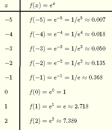
The natural exponential function f is an exponential functions with a base equal to Euler Constant e and is of the form

A table of values of followed by the graph of \( f \) are shown below.

Properties of the Natural Exponential Function \( f(x) = e^x \)

The natural exponential function has several properties that need to be highlighted.
Domain: \( (-\infty , +\infty) \)
Range: \( (0 , +\infty) \)
y intercept: \( (0,1) \)
Horizontal Asymptote: \( y = 0 \)
Monotonicity: increasing on the interval \( (-\infty , +\infty) \)
Continuity: continuous on the interval \( (-\infty , +\infty) \)
Differentiability: differentiable on the interval \( (-\infty , +\infty) \)
One to One Function: It is a one to one function and therefore has an inverse.
Inverse Function: The inverse of \( f(x) = e^x \) is the natural logarithm \( \ln (x) \)
Composition with its Inverse: \( e^{\ln(x)} = x \) for \( x \gt 0 \) and \( \ln(e^x) = x \)
Derivative: \( \dfrac{d e^x}{dx} = e^x \)
Indefinite integral: \( \int e^x dx = e^x + C \) , C is a constant of integration

Mathematical Models Using Exponential Function

Many mathematical models used in physics, engineering, chemistry, economics,..., are described by functions related to the natural exponential functions defined above.
Examples of some of the most used mathematical models based on natural exponential functions are listed below along with their graphs.

• Exponential Decay: \( f(x) = A e^{- kx} \) , \( k \gt 0 \)
  Example is shown below: \( y = e^{-0.5x} \) (red)
  
  
• Exponential Growth \( f(x) = A e^{kx} \) , \( k \gt 0 \)
  Example is shown below: \( y = e^{2x} \) (blue)
  
  
• Gaussian model: \( f(x) = A e^{-\left(\dfrac{x-a}{b}\right)^2} \)
  Example is shown below: \( f(x) = 3 e^{-\left(\dfrac{x-1}{2}\right)^2} \) (black)
  
  
  

Applications of the Natural Exponential Function - Examples with Detailed Solutions

We now discuss quantitatively some of the applications of the natural exponential functions.

Example 1: Population Growth Modeling
The population P of a city increases continuously according to the formula
\[ P = 120000 e^{0.01 t} \]
where t is the number of years after the year 2000.
What will be the population of this city in the year 2030?

Solution to Example 1
The number of years t between the years 2000 and 2030 is 30
Hence the population in 2030 is given by
\( P = 120000 e^{0.01 \times 30} = 161983\)

Example 2: Radioactive Material Decay Modeling
The amount \( A \) of a decaying radioactive material after \( t \) days is given by
\[ A = A_0 e^{-0.005 t} \]
where t is in days.
If the initial amount at t = 0 is 20 milligrams, then
a) what is the amount of radioactive material left after 30 days? Round your answer to the nearest hundredth.
b) how many days does it take the amount of the radioactive material to decay to 10 milligrams?

Solution to Example 2
a)
A = 20 at t = 0, hence
\( 20 = A_0 e^{-0.005 \times 0} = A_0 e^0 = A_0 \)
The formula for A may be written as
\( A = 20 e^{-0.005 t} \)
at t = 30 , A is given by
\( A = 20 e^{-0.005 \times 30} = 17.21 \) mg

b)
The amount is known, hence
\( 10 = 20 e^{-0.005 t} \)
we now need to find t, hence dividing both sides of the equation by 20.
\( e^{-0.005 t} = 10/20 = 0.5 \)
Take the natural logarithm ln of both sides
\( ln(e^{-0.005 t}) = ln(0.5) \)
Use the property \( \ln(e^x) = x \) to simplify left side of the equation
\( -0.005 t = ln(0.5) \)
\( t = \dfrac{ln(0.5)}{-0.005} = 138.63 \) days

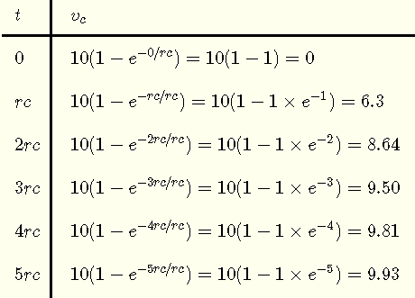
Example 3: R-C Circuit Modeling
In the circuit below, when the switch is on, the current i through the resistor r charges the capacitor c and hence creates a voltage across it. The voltage \( V_c \) across the capacitor c is given by a function including the natural exponential function as follows:
\[ V_c = V (1 - e^{-t/rc} ) \]


where \( t \) is in seconds, \( V \) in volts, \(r \) in Ohms, and \( c \) in Farads.
a) Let V = 10 volts and make a table of values of \( V_c \) as a function of \( t \) for values of \( t = 0, 2rc, 3rc, 4rc, 5rc, .... \). Round the answers to the nearest hundredth.
b) Use the values obtained in the table above to graph \( V_c \) as a function of \( t \).
c) Find the values of \( t \) in terms of rc for which \( V_c \) is equal to 9.99 volts.

Solution to Example 3
a)
b)


c)
We need to solve the equation
\( 9.99 = 10 (1 - e^{-t/rc} ) \)
expand the right side of the equation
\( 9.99 = 10 - 10 e^{-t/rc} \)
\( - 10 e^{-t/rc} = 9.99 - 10 \)
\( e^{-t/rc} = 0.001 \)
take the natural logarithm ln of both sides of the equation
\( ln(e^{-t/rc}) = ln(0.001) \)
evaluate the right side and use the property \( \ln(e^x) = x \) to simplify left side of the equation.
\( - t / rc = -6.90 \)
solve for t
\( t = 6.9 rc \)

Example 4: Continuous Compounding Interest
The balance B in a saving account after \( t \) years and continuous compounding of the annual interest r is given by
\[ B = P e^{r t}\]
where \( P \) is the principal.
An amout of \( \$ 10000 \) is invested at the rate \( r = 6.25\% \) and compounded continuously. How many years, after the initial deposit of $10000, will it take for the investment to double?

Solution to Example 4
Let t = 0 when the initial $10000 is deposited. Hence the balance B is given by
\[ B = 10000 e^{0.0625 t}\]
we now need to find t when B is double the initial deposit, hence \( B = 20000 \).
\( 20000 = 10000 e^{0.0625 t} \)
divide both sides by 10000 and simplify to obtain
\( 2 = e^{0.0625 t} \)
take the natural logarithm ln of both sides
\( ln( 2 ) = ln (e^{0.0625 t}) \)
Use the property \( \ln(e^x) = x \) to simplify right side of the equation and
\( 0.0625 t = ln(2) \)
\( t = ln(2) / 0.0625 \approx 11 \) years

More Compound Interest Problems with Detailed Solutions are included in this website.

More References and Links