Linear Programming and Optimization
What is Linear Programming?
A two-variable linear programming problem involves a linear function \( f(x,y) \) in two variables, called the objective function, along with a system of linear inequalities called constraints. These constraints define the feasible solution set (as explored in systems of inequalities with two variables).
Linear programming is an optimization method where we aim to find the values of variables \( x \) and \( y \) such that the function \( f(x,y) \) reaches a maximum or minimum value, depending on the application. These techniques are widely used in engineering, agriculture, medicine, finance, and economics.
Fundamental Theorems of Linear Programming
The solutions to a linear programming problem can be found using the following theorems:
- Theorem 1 (Vertex Theorem): The solution of a linear programming problem, if it exists, must occur at a vertex (corner point) of the feasible set associated with the constraints. If the optimal solution occurs at two adjacent vertices, then all points on the line segment joining those two vertices are also solutions.
- Theorem 2 (Bounded vs. Unbounded Sets): In a linear programming problem with a feasible set \( A \) and objective function \( f(x,y) = ax + by \):
- 1) If \( A \) is bounded (enclosed on all sides), then \( f(x,y) \) has both a maximum and a minimum at the vertices of \( A \).
- 2) If \( x \ge 0 \) and \( y \ge 0 \), and if \( A \) is unbounded (open-ended), and both \( a \) and \( b \) are positive, then \( f(x,y) \) will have a minimum at one or more vertices of \( A \), but no maximum.
Table of Contents
Worked Examples
Example 1: Finding a Maximum Value
Show Solution
Find the values of \( x \) and \( y \) that make the objective function \( z(x, y) = 2x + 4y \) a maximum subject to the conditions below. What is the value of \( z \) at these values of \( x \) and \( y \)?
\[ \begin{cases} x \ge 0 \\ y \ge 0 \\ y \le x + 1 \\ 4y + x \le 10 \\ y - x \ge -3 \end{cases} \]Solution
The feasible set (the region where all inequalities overlap) and its vertices are found by graphing the boundary lines. This specific region was derived in Example 3 of "Solving Systems of Inequalities in Two Variables".
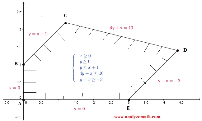
The vertices of the bounded region are:
- \( A(0, 0) \)
- \( B(0, 1) \)
- \( C\left(\frac{6}{5}, \frac{11}{5}\right) \)
- \( D\left(\frac{22}{5}, \frac{7}{5}\right) \)
- \( E(3, 0) \)
Evaluate the objective function \( z(x, y) = 2x + 4y \) at each of the 5 vertices:
- At \( A(0,0) \): \( z = 2(0) + 4(0) = 0 \)
- At \( B(0,1) \): \( z = 2(0) + 4(1) = 4 \)
- At \( C\left(\frac{6}{5}, \frac{11}{5}\right) \): \( z = 2\left(\frac{6}{5}\right) + 4\left(\frac{11}{5}\right) = \frac{12}{5} + \frac{44}{5} = \frac{56}{5} = 11.2 \)
- At \( D\left(\frac{22}{5}, \frac{7}{5}\right) \): \( z = 2\left(\frac{22}{5}\right) + 4\left(\frac{7}{5}\right) = \frac{44}{5} + \frac{28}{5} = \frac{72}{5} = \mathbf{14.4} \)
- At \( E(3,0) \): \( z = 2(3) + 4(0) = 6 \)
Conclusion: The function \( z \) has a maximum value of 14.4, which occurs at vertex \( D \) where \( x = \frac{22}{5} \) and \( y = \frac{7}{5} \).
Example 2: Finding a Minimum Value
Show Solution
Find the minimum value of \( z(x, y) = 4x + 7y \) where \( x \ge 0 \) and \( y \ge 0 \) subject to the following conditions:
\[ \begin{cases} 2x + 3y \ge 6 \\ x - \frac{y}{3} \le 4 \\ -2x + 2y \le 8 \\ x + \frac{5}{2}y \le 13 \end{cases} \]Solution
A vertex is determined by solving the system of equations corresponding to the boundary lines intersecting at that point.
- Solve \( 2x + 3y = 6 \) and \( x = 0 \) to find \( A(0, 2) \).
- Solve \( x = 0 \) and \( -2x + 2y = 8 \) to find \( B(0, 4) \).
- Solve \( -2x + 2y = 8 \) and \( x + \frac{5}{2}y = 13 \) to find \( C\left(\frac{6}{7}, \frac{34}{7}\right) \).
- Solve \( x + \frac{5}{2}y = 13 \) and \( x - \frac{y}{3} = 4 \) to find \( D\left(\frac{86}{17}, \frac{54}{17}\right) \).
- Solve \( x - \frac{y}{3} = 4 \) and \( y = 0 \) to find \( E(4, 0) \).
- Solve \( y = 0 \) and \( 2x + 3y = 6 \) to find \( F(3, 0) \).
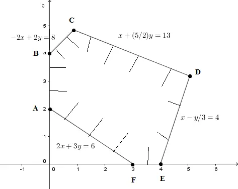
Evaluate \( z(x, y) = 4x + 7y \) at each vertex:
- At \( A(0, 2) \): \( z = 4(0) + 7(2) = 14 \)
- At \( B(0, 4) \): \( z = 4(0) + 7(4) = 28 \)
- At \( C\left(\frac{6}{7}, \frac{34}{7}\right) \): \( z = 4\left(\frac{6}{7}\right) + 7\left(\frac{34}{7}\right) = \frac{24 + 238}{7} = \frac{262}{7} \approx 37.43 \)
- At \( D\left(\frac{86}{17}, \frac{54}{17}\right) \): \( z = 4\left(\frac{86}{17}\right) + 7\left(\frac{54}{17}\right) = \frac{344 + 378}{17} = \frac{722}{17} \approx 42.47 \)
- At \( E(4, 0) \): \( z = 4(4) + 7(0) = 16 \)
- At \( F(3, 0) \): \( z = 4(3) + 7(0) = \mathbf{12} \)
Conclusion: The function \( z \) has a minimum value of 12, which occurs at vertex \( F \) where \( x = 3 \) and \( y = 0 \).
Example 3: Multiple (Infinite) Solutions
Show Solution
Find the maximum value of the function \( z = 3x + 3y \) where \( x \ge 0 \) and \( y \ge 0 \) subject to the conditions:
\[ \begin{cases} x \le 6 \\ y \le 7 \\ y \le -x + 9 \end{cases} \]Solution
The feasible set and boundary lines form a bounded polygon. The vertices are identified as follows:
- \( A(0, 0) \)
- \( B(0, 7) \) (from \( y = 7 \) and \( x = 0 \))
- \( C(2, 7) \) (Intersection of \( y = 7 \) and \( y = -x + 9 \))
- \( D(6, 3) \) (Intersection of \( x = 6 \) and \( y = -x + 9 \))
- \( E(6, 0) \) (from \( x = 6 \) and \( y = 0 \))
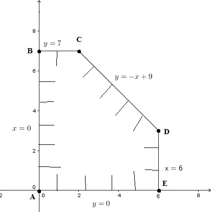
Evaluate \( z = 3x + 3y \) at each vertex:
- At \( A(0, 0) \): \( z = 3(0) + 3(0) = 0 \)
- At \( B(0, 7) \): \( z = 3(0) + 3(7) = 21 \)
- At \( C(2, 7) \): \( z = 3(2) + 3(7) = \mathbf{27} \)
- At \( D(6, 3) \): \( z = 3(6) + 3(3) = \mathbf{27} \)
- At \( E(6, 0) \): \( z = 3(6) + 3(0) = 18 \)
Observation: Function \( z = 3x + 3y \) has a maximum value at two adjacent vertices: \( C \) and \( D \). According to Theorem 1, all points lying on the line segment connecting \( C \) and \( D \) will also yield the maximum value of 27.
Notice that the objective function \( z = 3x + 3y \) can be factored as \( z = 3(x + y) \).
The boundary line segment connecting \( C \) and \( D \) is defined by the equation \( y = -x + 9 \), which can be rewritten as \( x + y = 9 \).
Substituting \( x + y = 9 \) into our factored objective function yields \( z = 3(9) = 27 \). Thus, any point on this boundary line provides the exact same maximum output.
Frequently Asked Questions
What is linear programming?
Linear programming is an optimization method that finds the maximum or minimum value of a linear objective function \( f(x,y) = ax + by \) subject to a system of linear inequality constraints. It is widely used in engineering, economics, agriculture, and finance.
Why does the optimal solution occur at a vertex?
The Vertex Theorem states that if a linear programming problem has an optimal solution, it occurs at a vertex (corner point) of the feasible region. This is because the objective function's level curves are parallel straight lines, which either first or last touch the feasible region at a vertex.
Can a linear programming problem have infinitely many optimal solutions?
Yes. If the objective function is parallel to one of the boundary lines of the feasible region, then every point on the line segment connecting two adjacent optimal vertices is also an optimal solution, producing infinitely many solutions.
What happens when the feasible region is unbounded?
If the feasible region is unbounded and the objective function's coefficients \( a \) and \( b \) are both positive with \( x \ge 0 \), \( y \ge 0 \), then the function will have a minimum at a vertex but no maximum. When the region is bounded, both a maximum and minimum always exist at vertices.
How do you find the vertices of the feasible region?
To find the vertices, solve the system of equations formed by each pair of boundary lines that intersect. The intersection point of two boundary lines is a vertex of the feasible region if it satisfies all other constraints.
References and Links on Linear Programming
- Systems of Inequalities in Two Variables
- Solving Inequalities with Two Variables
- Linear Programming Word Problems and Applications
- Find Systems of Inequalities from Graphs
- Linear Programming and Network Flows - 4th Edition - Mokhtar S. Bazaraa, John J. Jarvis, Hanif D. Sherali
- Introduction to Linear Optimization - 1st Edition - Dimitris Bertsimas, John N. Tsitsiklis
- Linear Programming: Foundations and Extensions - 5th Edition - Robert J. Vanderbei