What is Bayes' Theorem?
Starting from the Law of Total Probability:

For events \(A\) and mutually exclusive, exhaustive events \(E_1, E_2, ..., E_n\):
\[ P(A) = \sum_{i=1}^{n} P(A | E_i) P(E_i) \]
Using the definition of conditional probability:
\[ P(A) P(E_i | A) = P(E_i) P(A | E_i) \]
Solving for \( P(E_i | A) \):
\[ P(E_i | A) = \frac{P(E_i) P(A | E_i)}{P(A)} \]
Substituting \( P(A) \) from the Law of Total Probability gives Bayes' Theorem:
\[ P(E_i | A) = \frac{P(E_i) P(A | E_i)}{\sum_{i=1}^{n} P(A | E_i) P(E_i)} \]
Solved Examples of Bayes' Theorem
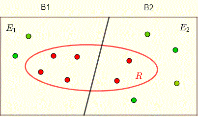
Example 1: Selecting Balls from Boxes
Problem: Two boxes contain colored balls:
- Box 1: 4 red, 2 green balls
- Box 2: 4 green, 2 red balls
The selection probabilities are: \( P(\text{Box 1}) = \frac{1}{3} \), \( P(\text{Box 2}) = \frac{2}{3} \). A box is chosen at random, then a ball is randomly selected from it.
- Given the ball is red, what is the probability it came from Box 1?
- Given the ball is red, what is the probability it came from Box 2?
- Compare and interpret the results.
Solution
Define events: \( B_1 \)=select Box 1, \( B_2 \)=select Box 2, \( R \)=select red ball.
Given probabilities:
\[ P(B_1) = \frac{1}{3}, \quad P(B_2) = \frac{2}{3} \]
\[ P(R|B_1) = \frac{4}{6} = \frac{2}{3}, \quad P(R|B_2) = \frac{2}{6} = \frac{1}{3} \]
Part (a): Using Bayes' Theorem:
\[ P(B_1 | R) = \frac{P(R|B_1)P(B_1)}{P(R|B_1)P(B_1) + P(R|B_2)P(B_2)} = \frac{\frac{2}{3} \cdot \frac{1}{3}}{\frac{2}{3} \cdot \frac{1}{3} + \frac{1}{3} \cdot \frac{2}{3}} = \frac{1}{2} \]
Part (b): Similarly:
\[ P(B_2 | R) = \frac{P(R|B_2)P(B_2)}{P(R|B_1)P(B_1) + P(R|B_2)P(B_2)} = \frac{\frac{1}{3} \cdot \frac{2}{3}}{\frac{2}{3} \cdot \frac{1}{3} + \frac{1}{3} \cdot \frac{2}{3}} = \frac{1}{2} \]
Part (c): The probabilities are equal (\( \frac{1}{2} \)) despite Box 1 having more red balls. This occurs because Box 2 is twice as likely to be selected initially. Bayes' Theorem incorporates all prior information.
Example 2: Disease Testing Accuracy
Problem: 1% of a population has a disease. A test is 95% accurate on diseased individuals and 98% accurate on disease-free individuals (2% false positive). If a random person tests positive, what is the probability they actually have the disease?
Solution
Define: \( D \)=has disease, \( ND \)=no disease, \( TP \)=tests positive.

Given: \( P(D) = 0.01 \), \( P(ND) = 0.99 \), \( P(TP|D) = 0.95 \), \( P(TP|ND) = 0.02 \).
\[ P(D | TP) = \frac{P(TP|D)P(D)}{P(TP|D)P(D) + P(TP|ND)P(ND)} = \frac{0.95 \cdot 0.01}{0.95 \cdot 0.01 + 0.02 \cdot 0.99} \approx 0.324 \]
Interpretation: Only about 32.4% probability that a positive-testing person actually has the disease. This low value arises because the disease is rare (1%), making false positives from the large healthy population significant.
Example 3: Factory Defect Rates
Problem: Three factories produce light bulbs:
- Factory A: 20% production, 2% defective
- Factory B: 50% production, 1% defective
- Factory C: 30% production, 3% defective
A randomly purchased bulb is defective. What is the probability it came from Factory B?
Solution
Define events: \( A, B, C \) (bulb from respective factory), \( D \)=defective.
Given: \( P(A)=0.2, P(B)=0.5, P(C)=0.3 \), \( P(D|A)=0.02, P(D|B)=0.01, P(D|C)=0.03 \).
\[ P(B | D) = \frac{P(D|B)P(B)}{P(D|A)P(A) + P(D|B)P(B) + P(D|C)P(C)} \]
\[ = \frac{0.01 \cdot 0.5}{0.02 \cdot 0.2 + 0.01 \cdot 0.5 + 0.03 \cdot 0.3} = \frac{0.005}{0.018} \approx 0.2778 \]
Despite producing 50% of bulbs, Factory B contributes only ~27.8% to defective bulbs because of its lower defect rate (1%).
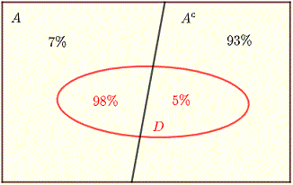
Example 4: Radar Detection System
Problem: A radar detects aircraft with 98% probability if present. If no aircraft, it falsely reports detection 5% of the time. Aircraft presence probability is 7%.
- Given detection, probability no aircraft is present?
- Given detection, probability aircraft is present?
- Given no detection, probability aircraft is present?
- Given no detection, probability no aircraft is present?
Solution
Define: \( A \)=aircraft present, \( A^c \)=no aircraft, \( D \)=detected, \( D^c \)=not detected.
Given: \( P(A)=0.07, P(A^c)=0.93 \), \( P(D|A)=0.98, P(D|A^c)=0.05 \).
Part (a):
 \[ P(A^c | D) = \frac{P(D|A^c)P(A^c)}{P(D|A)P(A) + P(D|A^c)P(A^c)} = \frac{0.05 \cdot 0.93}{0.98 \cdot 0.07 + 0.05 \cdot 0.93} \approx 0.4040 \]
Part (b):
\[ P(A | D) = \frac{P(D|A)P(A)}{P(D|A)P(A) + P(D|A^c)P(A^c)} = \frac{0.98 \cdot 0.07}{0.98 \cdot 0.07 + 0.05 \cdot 0.93} \approx 0.5960 \]
Part (c): First find: \( P(D^c|A)=1-0.98=0.02 \), \( P(D^c|A^c)=1-0.05=0.95 \).
 \[ P(A | D^c) = \frac{P(D^c|A)P(A)}{P(D^c|A)P(A) + P(D^c|A^c)P(A^c)} = \frac{0.02 \cdot 0.07}{0.02 \cdot 0.07 + 0.95 \cdot 0.93} \approx 0.0016 \]
Part (d):
\[ P(A^c | D^c) = \frac{P(D^c|A^c)P(A^c)}{P(D^c|A^c)P(A^c) + P(D^c|A)P(A)} = \frac{0.95 \cdot 0.93}{0.95 \cdot 0.93 + 0.02 \cdot 0.07} \approx 0.9984 \]
Visual Aid: All probabilities can be organized in a tree diagram:
