Dada una base
es una base ortogonal para el subespacio V .
La base ortonormal Y0 se obtiene dividiendo cada vector de la base Y por su norma.
El proceso de Gram Schmidt se utiliza para producir una Base Ortonormal para un subespacio.
Dada una base
![]() para el subespacio V ,
la base
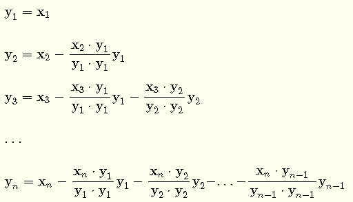
para el subespacio V ,
la base
![]() donde
donde
es una base ortogonal para el subespacio V .
![]()
La base ortonormal Y0 se obtiene dividiendo cada vector de la base Y por su norma.
Ejemplo 1
El subespacio \( V \) está definido por span\( \{\textbf{v}_1 , \textbf{v}_2 \} \) donde \( \textbf{v}_1 \) y \(\textbf{v}_2 \) son vectores columna dados por
\( \textbf{v}_1 =
\begin{bmatrix}
1\\
2 \\
0
\end{bmatrix}
\) y \( \textbf{v}_2 =
\begin{bmatrix}
-2 \\
-4 \\
-4
\end{bmatrix}
\)
Utilice el proceso de Gram Schmidt definido anteriormente para determinar una base ortonormal \( Y_O \) para \( V \)
Solución al Ejemplo 1
Sea \( Y = \{ \textbf{y}_1 , \textbf{y}_2 \} \) la base ortogonal a determinar. Según las fórmulas anteriores, escribimos
\( \textbf {y}_1 = \textbf {v}_1 = \begin{bmatrix}
1\\
2 \\
0
\end{bmatrix}
\)
\( \textbf {y}_2 = \textbf {v}_2 - \dfrac{\textbf {v}_2 \cdot \textbf {y}_1}{\textbf {y}_1 \cdot \textbf {y}_1} \textbf {y}_1 \)
Evaluar el producto interno en el numerador y denominador
\( \dfrac{\textbf {v}_2 \cdot \textbf {y}_1}{\textbf {y}_1 \cdot \textbf {y}_1} = \dfrac{\begin{bmatrix}
-2 \\
-4 \\
-4
\end{bmatrix} \cdot \begin{bmatrix}
1\\
2 \\
0
\end{bmatrix} }{ \begin{bmatrix}
1\\
2 \\
0
\end{bmatrix} \cdot \begin{bmatrix}
1\\
2 \\
0
\end{bmatrix} } = \dfrac{-10}{5} = -2\)
Sustituir lo anterior y evaluar \( \textbf {y}_2 \)
\( \textbf {y}_2 = \begin{bmatrix}
-2 \\
-4 \\
-4
\end{bmatrix}
- (-2)
\begin{bmatrix}
1\\
2 \\
0
\end{bmatrix}
= \begin{bmatrix}
0\\
0 \\
-4
\end{bmatrix}
\)
Por lo tanto \( Y = \left \{\begin{bmatrix}
1\\
2 \\
0
\end{bmatrix}
,
\begin{bmatrix}
0\\
0 \\
-4
\end{bmatrix} \right \} \)
La base ortonormal \( Y_O \) se obtiene dividiendo cada vector de la base \( Y \) por su norma.
\( Y_O = \left \{ \dfrac{1}{\sqrt 3}\begin{bmatrix}
1\\
2 \\
0
\end{bmatrix}
,
\dfrac{1}{4} \begin{bmatrix}
0\\
0 \\
-4
\end{bmatrix} \right \} \)
Nota que
1) \( Y = \{ \textbf {y}_1 , \textbf {y}_2 \} \) es una base para \( V \) porque es una combinación lineal de \( \textbf {v}_1 \) y \( \textbf {v}_2 \).
Sabemos que \( y_1 = v_1 \) y se puede demostrar fácilmente que \( y_2 = 2 v_1 + v_2 \)
Por lo tanto span \( \{ \textbf {v}_1, \textbf{v}_2 \} \) = span \( \{ \textbf {y}_1, \textbf{y}_2 \} \)
2) el producto interno de \( \textbf {y}_1 \) y \( \textbf {y}_2 \) dado por
\(
\begin{bmatrix}
1\\
2 \\
0
\end{bmatrix}
\cdot
\begin{bmatrix}
0\\
0 \\
-4
\end{bmatrix}
= 0
\)
significa que \( \textbf {y}_1 \) y \( \textbf {y}_2 \) son ortogonales y por lo tanto \( Y \) es una base ortogonal para \( V \)
Ejemplo 2
El subespacio \( V \) está definido por span\( \{\textbf{v}_1 , \textbf{v}_2 , \textbf{v}_3 , \textbf{v}_4\} \) donde
\( \textbf{v}_1 =
\begin{bmatrix}
-1\\
-1 \\
2 \\
2\\
3
\end{bmatrix}
\) , \( \textbf{v}_2 =
\begin{bmatrix}
1 \\
1 \\
1\\
1\\
0
\end{bmatrix}
\) ,
\( \textbf{v}_3 =
\begin{bmatrix}
0 \\
0 \\
-1\\
-1\\
0
\end{bmatrix}
\)
,
\( \textbf{v}_4 =
\begin{bmatrix}
0 \\
0 \\
0\\
1\\
1
\end{bmatrix}
\)
Utilice el proceso de Gram Schmidt definido anteriormente para determinar una base ortonormal \( Y_O \) para \( V \)
Solución al Ejemplo 2
Sea \( Y = \{\textbf{y}_1,\textbf{y}_2,\textbf{y}_3,\textbf{y}_4\} \) la base ortogonal a determinar. Usando las fórmulas anteriores, escribimos
\( \textbf {y}_1 = \textbf {v}_1 =
\begin{bmatrix}
-1\\
-1 \\
2 \\
2\\
3
\end{bmatrix}
\)
\( \textbf {y}_2 = \textbf {v}_2 - \dfrac{\textbf {v}_2 \cdot \textbf {y}_1}{\textbf {y}_1 \cdot \textbf {y}_1} \textbf {y}_1 \)
Evaluar el producto interno en el numerador y denominador
\( \dfrac{\textbf {v}_2 \cdot \textbf {y}_1}{\textbf {y}_1 \cdot \textbf {y}_1} = \dfrac{\begin{bmatrix}
1 \\
1 \\
1\\
1\\
0
\end{bmatrix} \cdot \begin{bmatrix}
-1\\
-1 \\
2 \\
2\\
3
\end{bmatrix} }{ \begin{bmatrix}
-1\\
-1 \\
2 \\
2\\
3
\end{bmatrix} \cdot \begin{bmatrix}
-1\\
-1 \\
2 \\
2\\
3
\end{bmatrix} } = \dfrac{2}{19} \)
Sustituir lo anterior y evaluar \( \textbf {y}_2 \)
\( \textbf {y}_2 = \begin{bmatrix}
1 \\
1 \\
1\\
1\\
0
\end{bmatrix}
- \dfrac{2}{19}
\begin{bmatrix}
-1\\
-1 \\
2 \\
2\\
3
\end{bmatrix}
=
\begin{bmatrix}
\frac{21}{19}\\
\frac{21}{19}\\
\frac{15}{19}\\
\frac{15}{19}\\
-\frac{6}{19}\end{bmatrix}
\)
Nota que si multiplicamos \( \textbf{y}_2 \) por cualquier número distinto de cero, no cambiaría la base. Por lo tanto, multiplicamos \( \textbf{y}_2 \) por \( \dfrac{19}{3} \) y simplificamos para obtener
\( \textbf{y'}_2 = \dfrac{19}{3} \begin{bmatrix}
\frac{21}{19}\\
\frac{21}{19}\\
\frac{15}{19}\\
\frac{15}{19}\\
-\frac{6}{19}\end{bmatrix} =
\begin{bmatrix}
7\\
7\\
5\\
5\\
-2
\end{bmatrix}
\)
Ahora usamos el vector \( \textbf {y'}_2 \) en lugar de \( \textbf {y}_2 \) en las fórmulas para \( \textbf {y}_3 \).
\( \textbf {y}_3 = \textbf {v}_3 - \dfrac{\textbf {v}_3 \cdot \textbf {y}_1}{\textbf {y}_1 \cdot \textbf {y}_1} \textbf {y}_1
- \dfrac{\textbf {v}_3 \cdot \textbf {y'}_2}{\textbf {y'}_2 \cdot \textbf {y'}_2} \textbf {y'}_2 \)
Sustituir
\( \textbf {y}_3 = \begin{bmatrix}
0 \\
0 \\
-1\\
-1\\
0
\end{bmatrix} -
\dfrac{\begin{bmatrix}
0 \\
0 \\
-1\\
-1\\
0
\end{bmatrix} \cdot \begin{bmatrix}
-1\\
-1 \\
2 \\
2\\
3
\end{bmatrix} }{\begin{bmatrix}
-1\\
-1 \\
2 \\
2\\
3
\end{bmatrix} \cdot \begin{bmatrix}
-1\\
-1 \\
2 \\
2\\
3
\end{bmatrix} } \begin{bmatrix}
-1\\
-1 \\
2 \\
2\\
3
\end{bmatrix}
\)
\(
- \dfrac{\begin{bmatrix}
0 \\
0 \\
-1\\
-1\\
0
\end{bmatrix} \cdot \begin{bmatrix}
7\\
7\\
5\\
5\\
-2
\end{bmatrix} }{\begin{bmatrix}
7\\
7\\
5\\
5\\
-2
\end{bmatrix} \cdot \begin{bmatrix}
7\\
7\\
5\\
5\\
-2
\end{bmatrix} } \begin{bmatrix}
7\\
7\\
5\\
5\\
-2
\end{bmatrix} =
\begin{pmatrix}\frac{1}{4}\\ \frac{1}{4}\\ -\frac{1}{4}\\ -\frac{1}{4}\\ \frac{1}{2}\end{pmatrix}
\)
Multiplicamos \( \textbf {y}_3 \) por 4 para reemplazarlo por un vector sin fracciones.
\( \textbf {y'}_3 = 4 \textbf {y}_3 = \begin{bmatrix}
1\\
1 \\
-1 \\
-1\\
2
\end{bmatrix}\)
Usamos \( \textbf {y'}_3 \) en lugar de \( \textbf {y}_3 \) en las fórmulas
\( \textbf {y}_4 = \textbf {v}_4 - \dfrac{\textbf {v}_4 \cdot \textbf {y}_1}{\textbf {y}_1 \cdot \textbf {y}_1} \textbf {y}_1
- \dfrac{\textbf {v}_4 \cdot \textbf {y'}_2}{\textbf {y'}_2 \cdot \textbf {y'}_2} \textbf {y'}_2
- \dfrac{\textbf {v}_4\cdot \textbf {y'}_3}{\textbf {y'}_3 \cdot \textbf {y'}_3} \textbf {y'}_3 \)
Sustituir
\( \textbf {y}_4 = \begin{bmatrix}
0 \\
0 \\
0\\
1\\
1
\end{bmatrix} - \dfrac{\begin{bmatrix}
0 \\
0 \\
0\\
1\\
1
\end{bmatrix} \cdot \begin{bmatrix}
-1\\
-1 \\
2 \\
2\\
3
\end{bmatrix}}{\begin{bmatrix}
-1\\
-1 \\
2 \\
2\\
3
\end{bmatrix} \cdot \begin{bmatrix}
-1\\
-1 \\
2 \\
2\\
3
\end{bmatrix}} \begin{bmatrix}
-1\\
-1 \\
2 \\
2\\
3
\end{bmatrix}
\)
-
\(
\dfrac{\begin{bmatrix}
0 \\
0 \\
0\\
1\\
1
\end{bmatrix} \cdot \begin{bmatrix}
7\\
7\\
5\\
5\\
-2
\end{bmatrix}}{\begin{bmatrix}
7\\
7\\
5\\
5\\
-2
\end{bmatrix} \cdot \begin{bmatrix}
7\\
7\\
5\\
5\\
-2
\end{bmatrix}} \begin{bmatrix}
7\\
7\\
5\\
5\\
-2
\end{bmatrix}
\\ \quad \quad
- \dfrac{\begin{bmatrix}
0 \\
0 \\
0\\
1\\
1
\end{bmatrix} \cdot \begin{bmatrix}
1\\
1 \\
-1 \\
-1\\
2
\end{bmatrix}}{\begin{bmatrix}
1\\
1 \\
-1 \\
-1\\
2
\end{bmatrix} \cdot \begin{bmatrix}
1\\
1 \\
-1 \\
-1\\
2
\end{bmatrix}} \begin{bmatrix}
1\\
1 \\
-1 \\
-1\\
2
\end{bmatrix} = \begin{pmatrix}0\\ 0\\ -\frac{1}{2}\\ \frac{1}{2}\\ 0\end{pmatrix}\)
Multiplicamos \( \textbf {y}_4 \) por 2 para obtener
\( \textbf {y'}_4 = 2 \textbf {y}_4 = \begin{bmatrix}
0\\
0\\
-1 \\
1\\
0
\end{bmatrix}\)
Por lo tanto, una base ortogonal para el subespacio \( V \) se puede escribir como
\( Y = \left \{ \textbf {y}_1 , \textbf {y'}_2 , \textbf {y'}_3 , \textbf {y'}_4 \right \} = \left \{ \begin{bmatrix}
-1\\
-1 \\
2 \\
2\\
3
\end{bmatrix} ,
\begin{bmatrix}
7\\
7\\
5\\
5\\
-2
\end{bmatrix}
,
\begin{bmatrix}
1\\
1 \\
-1 \\
-1\\
2
\end{bmatrix}
,
\begin{bmatrix}
0\\
0\\
-1 \\
1\\
0
\end{bmatrix}
\right \} \)
La base ortonormal \( Y_O \) se obtiene dividiendo cada vector de la base \( Y \) por su norma.
\( Y_O = \left \{ \dfrac{1}{\sqrt {19}} \begin{bmatrix}
-1\\
-1 \\
2 \\
2\\
3
\end{bmatrix} ,
\dfrac{1}{2\sqrt{38}}
\begin{bmatrix}
7\\
7\\
5\\
5\\
-2
\end{bmatrix}
,
\dfrac{1}{2\sqrt{2}}
\begin{bmatrix}
1\\
1 \\
-1 \\
-1\\
2
\end{bmatrix}
,
\dfrac{1}{\sqrt{2}}
\begin{bmatrix}
0\\
0\\
-1 \\
1\\
0
\end{bmatrix}
\right \} \)
Para comprobar que la base \( Y \) obtenida genera el mismo subespacio que la base dada \( V \), reducimos por filas la matriz
\(
\begin{bmatrix}
V | Y
\end{bmatrix}
=
\begin{bmatrix}-1&1&0&0&-1&7&1&0\\ \:\:\:-1&1&0&0&-1&7&1&0\\ \:\:\:2&1&-1&0&2&5&-1&-1\\ \:\:\:2&1&-1&1&2&5&-1&1\\ \:\:\:3&0&0&1&3&-1&2&0\end{bmatrix}
\)
para obtener
\(
\begin{bmatrix}1&0&0&0&1&-\frac{1}{3}&\frac{2}{3}&-\frac{2}{3}\\ 0&1&0&0&0&\frac{20}{3}&\frac{5}{3}&-\frac{2}{3}\\ 0&0&1&0&0&1&4&-1\\ 0&0&0&1&0&0&0&2\\ 0&0&0&0&0&0&0&0\end{bmatrix}
\)
y concluimos de lo anterior que
\( y_1 = v_1 \)
\( y_2 = - \dfrac {1}{3} v_1 + \dfrac{20}{3} v_2 + v_3\)
\( y_3 = \dfrac {2}{3} v_1 + \dfrac{5}{3} v_2 + 4 v_3\)
\( y_4 = - \dfrac {2}{3} v_1 - \dfrac{2}{3} v_2 - v_3 + 2 v_4\)
Los resultados anteriores muestran que span \( \{ \textbf {v}_1, \textbf{v}_2,\textbf{v}_3 ,\textbf{v}_4 \} \) = span \( \{ \textbf {y}_1, \textbf{y}_2, \textbf{y}_3 , \textbf{y}_3 \} \)
Usando el producto interno, se puede demostrar fácilmente que \( Y \) es una base ortogonal.