Quartiles and box plots
Quartiles split a given a data set of real numbers x1, x2, x3 ... xN into four groups, sorted in ascending order, and each group includes approximately 25% (or a quarter) of all the data values included in the data set.
Let Q1 be the lower quartile, Q2 be the median and Q3 be the be the upper quartile. The four groups of data values are defined by the intervals:
Group 1: From the minimum data value to Q1 , Q1 is also called the 25th percentile because 25% of the data values in the data set are below Q1
Group 2: From Q1 to Q2 , Q2 is also called the 50th percentile because 50% of the data values in the data set are below Q2
Group 3: From Q2 to Q3 , Q3 is also called the 75th percentile because 75% of the data values in the data set are below Q3
Group 4: From Q3 to maximum data value.

Methods in Calculating Quartiles
There are different methods to calculate the quartiles. Two methods, that differ only if the number of data values is odd, will described and used.
For both methods, you start by finding the median which is Q2.
You then divide the ordered data set into two halves: a lower half and an upper half. If the number of data values N is even, the split is straightforward. However if H is odd, there are two methods in creating the two halves
First method
Split the data set into two halves without including the median. The lower quartile Q1 is the median of the lower half and the upper quartile is the median of the upper half.
Second method
Split the data set into two halves including the median in both halves
The lower quartile Q1 is the median of the lower half and the upper quartile is the median of the upper half.
Examples on Computing Quartiles and Drawing Box Plot
Example 1
Calculate the quartiles of the data set: 20 , 2 , 1 , 12 , 4 , 8 , 9 , 6 and draw the box plot.
Solution to Example 1
We first order the data set in ascending order
1 , 2 , 4 , 6 , 8 , 9 , 12 , 20
Find the median Q2 of the given data set: Q2 = (6 + 8) / 2 = 7
The number N of data values is equal to 8 and therefore even; we split the data set into two halves
lower half: 1 , 2 , 4 , 6
Upper half: 8 , 9 , 12 , 20
The lower quartile Q1 is equal to the median of the lower half; hence
Q1 = (2 + 4) / 2 = 3
The upper quartile Q3 is equal to the median of the upper half; hence
Q3 = (9 + 12) / 2 = 10.5
The quartiles, the minimum and maximum data values are plotted together along with the data values (in blue) to create what is called a box plot as shown below. The data set is split into four groups as described above with the two groups in the middle from Q1 to Q3 making the box and the outside groups from the minimum to Q1 and from Q3 to the maximum making the whiskers.
Group 1: From the minimum data value to Q1
Group 2: From Q1 to Q2
Group 3: From Q2 to Q3
Group 4: From Q3 to maximum data value.
We can easily check that each group contains 2 data values out of a total of 8 which is one quarter or 25% of the data values.

Box plots are a five-number summary that includes the minimum and maximum data values, the median and lower and upper quartiles. They can be useful in understanding how is data distributed in a given set and give qualitatif information about the spread of the data.
Example 2
The scores of a class in a Math exam are: 55 , 35 , 60 , 86 , 65 , 75 , 83 , 88 , 88 , 90 , 95 , 96 , 98. Calculate the quartiles of the scores and draw a box plot.
Solution to Example 2
We first order the data set in ascending order
35 , 55 , 60 , 65 , 75 , 83 , 86 , 88 , 88 , 90 , 95 , 96 , 98
Find the median Q2 of the given data set: Q2 = 86
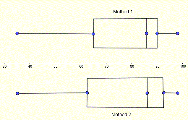
The number N of data values is equal to 13 and therefore odd; we will use the two methods described above. Method 1: Split the scores into two halves including the median 86
lower half: 35 , 55 , 60 , 65 , 75 , 83 , 86
Upper half: 86 , 88 , 88 , 90 , 95 , 96 , 98
The lower quartile Q1 is equal to the median of the lower half; hence
Q1 = 65
The upper quartile Q3 is equal to the median of the upper half; hence
Q3 = 90
The quartiles, the minimum and maximum data values are plotted together to create what is called a box plot as shown below. The data set is split into four groups as described above
Method 2: Split the scores into two halves not including the median 86
lower half: 35 , 55 , 60 , 65 , 75 , 83
Upper half: 88 , 88 , 90 , 95 , 96 , 98
The lower quartile Q1 is equal to the median of the lower half;
Q1 = (60 + 65) / 2 = 62.5
The upper quartile Q3 is equal to the median of the upper half; hence
Q3 = (90 + 95) / 2 = 92.5
The box plots with quartiles, the minimum and maximum data values are plotted below for the two methods.

Examples on Reading Quartiles from Box plots
Example 3
The box plots of the scores in an exam of classes A, B, C and D are shown below. The number of students in each of the classes A, B,C and D are 12, 19, 22 and 28 respectively.

Use the box plots to answer the following questions
a) Determine the minimum and maximum scores, the lower and upper quartiles, the median, the range and interquartile range (IQR) of each class.
b) Which class has the highest score?
c) Which class has the lowest score?
d) How many students scored above the median in each class?
e) How many students scored below the lower quartile in each class?
f) How many students scored the lower quartile and the maximum in each class?
g) Using the range and interquartile ranges, which class has the highest dispersion and which class has the lowest dispersion of scores?
Solution to Example 3
a)
Range = maximum data value - minimum data value
Interquartile range (IQR) = Q3 - Q1
|
minimum |
maximum |
Q1 |
Q3 |
Q2 |
Range |
IQR |
| Class A |
50 |
94 |
64 |
90 |
85 |
44 |
26 |
| Class B |
20 |
100 |
60 |
94 |
76 |
80 |
34 |
| Class C |
41 |
98 |
65 |
90 |
85 |
57 |
25 |
| Class D |
30 |
98 |
60 |
90 |
82 |
68 |
30 |
b)
Class B has the highest score of 100
c)
Class B has the lowest score of 20
d)
The median splits the ordered scores into two halves and therefore half the class scores above the median
class A: (1/2) total = (1/2) 12 = 6 students
class B: (1/2) total = (1/2) 19 = 9.5 , round to 10 students (number of students must be an integer)
class C: (1/2) total = (1/2) 22 = 11 students
class D: (1/2) total = (1/2) 28 = 14 students
e)
Quartiles splits the data set (scores in this example) into 4 groups with 1/4 each. Hence, for each class, one quarter of the scores are below the lower quartile
class A: (1/4) total = (1/4) 12 = 3 students
class B: (1/4) total = (1/4) 19 = 4.75 , round to 5 students (number of students must be an integer)
class C: (1/4) total = (1/4) 22 = 5.5 , round to 6 students (number of students must be an integer)
class D: (1/4) total = (1/4) 28 = 7 students
f)
Quartiles splits the data set (scores in this example) into 4 groups with 1/4 each. Hence, for each class, 3/4 quarters of the scores are between the lower quartile and the maximum (or above the lower quartile)
class A: (3/4) total = (3/4) 12 = 9 students
class B: (3/4) total = (3/4) 19 = 14.25, round to 14 students (number of students must be an integer)
class C: (3/4) total = (3/4) 22 = 16.5 , round to 17 students (number of students must be an integer|)
class D: (3/4) total = (3/4) 28 = 21 students
g)
Class A has the smallest range and interquartile range; 44 and 26 respectively.
Class B has the largest range and interquartile rangep; 80 and 34 respectively.
Using the box plots and the range and interquartile range, we may conclude that the scores in class A has the smallest dispersion and the scores in class B has the largest dispersion.
More References and Links
Quartile
Mean, Median and Mode
standard deviation
Mean and Standard deviation.
John W. Tukey (1977). Exploratory Data Analysis. Addison-Wesley.


