Nous présentons des exemples où les équations différentielles sont largement appliquées pour modéliser des phénomènes naturels, des systèmes d'ingénierie et de nombreuses autres situations.
Application 1 : Croissance exponentielle - Population
Soit \( P(t) \) une quantité qui augmente avec le temps \( t \) et dont le taux d'augmentation est proportionnel à cette même quantité \( P \) de la manière suivante :
\[ \frac{dP}{dt} = kP \]où \( \frac{dP}{dt} \) est la première dérivée de \( P \), \( k > 0 \) et \( t \) est le temps.
La solution de cette équation différentielle du premier ordre est donnée par :
\[ P(t) = A e^{kt} \]où \( A \) est une constante non nulle.
Si \( P = P_0 \) à \( t = 0 \), alors :
\[ P_0 = A e^0 \]ce qui donne \( A = P_0 \). La forme finale de la solution est donnée par :
En supposant que \( P_0 \) est positif et puisque \( k \) est positif, \( P(t) \) est une exponentielle croissante. L'équation \( \frac{dP}{dt} = kP \) est également appelée modèle de croissance exponentielle.
Application 2 : Décroissance exponentielle - Matière radioactive
Soit \( M(t) \) la quantité d'un produit qui diminue avec le temps \( t \) et dont le taux de diminution est proportionnel à la quantité \( M \) de la manière suivante :
\[ \frac{dM}{dt} = -kM \]où \( \frac{dM}{dt} \) est la première dérivée de \( M \), \( k > 0 \) et \( t \) est le temps.
Résolvons cette équation différentielle du premier ordre pour obtenir :
\[ M(t) = A e^{-kt} \]où \( A \) est une constante non nulle.
Si nous supposons que \( M = M_0 \) à \( t = 0 \), alors :
\[ M_0 = A e^0 \]ce qui donne \( A = M_0 \). La solution peut s'écrire ainsi :
En supposant que \( M_0 \) est positif et puisque \( k \) est positif, \( M(t) \) est une exponentielle décroissante. L'équation \( \frac{dM}{dt} = -kM \) est également appelée modèle de décroissance exponentielle.
Application 3 : Objet en chute libre
Un objet est lâché d'une certaine hauteur à l'instant \( t = 0 \). Si \( h(t) \) est la hauteur de l'objet au temps \( t \), \( a(t) \) l'accélération et \( v(t) \) la vitesse, les relations entre \( a \), \( v \) et \( h \) sont les suivantes :
\[ a(t) = \frac{dv}{dt}, \quad v(t) = \frac{dh}{dt} \]Pour un objet en chute libre, \( a(t) \) est constant et égal à \( g = -9.8 \, \text{m/s}^2 \).
En combinant les équations différentielles ci-dessus, nous pouvons facilement déduire l'équation suivante :
\[ \frac{d^2h}{dt^2} = g \]Intégrons les deux côtés de cette équation pour obtenir :
\[ \frac{dh}{dt} = gt + v_0 \]Intégrons une seconde fois pour obtenir :
L'équation ci-dessus décrit la hauteur d'un objet en chute libre, à partir d'une hauteur initiale \( h_0 \) et à une vitesse initiale \( v_0 \), en fonction du temps.
Application 4 : Loi de refroidissement de Newton
C'est un modèle qui décrit mathématiquement le changement de température d'un objet dans un environnement donné. La loi stipule que le taux de variation (dans le temps) de la température est proportionnel à la différence entre la température \( T \) de l'objet et la température \( T_e \) de l'environnement qui entoure l'objet :
\[ \frac{dT}{dt} = -k(T - T_e) \]Soit \( x = T - T_e \) de sorte que \( \frac{dx}{dt} = \frac{dT}{dt} \).
En utilisant ce changement de variable, l'équation différentielle devient :
\[ \frac{dx}{dt} = -kx \]La solution de cette équation différentielle est donnée par :
\[ x = A e^{-kt} \]Substituons \( x \) par \( T - T_e \) :
\[ T - T_e = A e^{-kt} \]Supposons qu'à \( t = 0 \), la température \( T = T_0 \) :
\[ T_0 - T_e = A e^0 \]ce qui donne \( A = T_0 - T_e \).
L'expression finale de \( T(t) \) est donnée par :
Cette dernière expression montre comment la température \( T \) de l'objet évolue au fil du temps.
Application 5 : Circuit RL
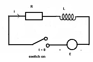
Considérons le circuit RL (résistance R et inductance L) illustré ci-dessus. À \( t = 0 \), l'interrupteur est fermé et le courant traverse le circuit. Les lois de l'électricité stipulent que la tension aux bornes d'une résistance de résistance \( R \) est égale à \( R i \), et la tension aux bornes d'une inductance \( L \) est donnée par \( L \frac{di}{dt} \) (où \( i \) est le courant). Une autre loi fournit une équation reliant toutes les tensions du circuit de la manière suivante :
\[ L \frac{di}{dt} + Ri = E, \quad \text{où } E \text{ est une tension constante} \]Résolvons l'équation différentielle ci-dessus, qui peut s'écrire ainsi :
\[ L \frac{\frac{di}{dt}}{E - Ri} = 1 \]Ceci peut s'écrire :
\[ -\frac{L}{R} \frac{-Rdi}{E - Ri} = dt \]Intégrons les deux côtés :
\[ -\frac{L}{R} \ln(E - Ri) = t + c, \quad c \text{ constante d'intégration} \]Trouvons la constante \( c \) en posant \( i = 0 \) à \( t = 0 \) (quand l'interrupteur est fermé), ce qui donne :
\[ c = -\frac{L}{R} \ln(E) \]Substituons \( c \) dans la solution :
\[ -\frac{L}{R} \ln(E - Ri) = t - \frac{L}{R} \ln(E) \]Ceci peut s'écrire :
\[ \frac{L}{R} \ln\left(\frac{E}{E - Ri}\right) = t \]Passons à la forme exponentielle :
\[ \frac{E}{E - Ri} = e^{t(R/L)} \]Résolvons pour \( i \) afin d'obtenir :
Le modèle de départ du circuit est une équation différentielle qui, une fois résolue, donne une expression du courant dans le circuit en fonction du temps.