Un tutoriel sur la façon d'utiliser les première et seconde dérivées, en analyse, pour étudier les propriétés des graphiques de fonctions.
Dans ce qui suit, \( C \) représente la constante d'intégration le cas échéant.
Théorèmes
Pour tracer des fonctions en analyse, nous passons d'abord en revue plusieurs théorèmes. Trois théorèmes sont utilisés pour trouver les maxima et minima en utilisant les première et seconde dérivées, et ils sont combinés ici avec deux théorèmes supplémentaires pour étudier des graphiques de fonctions complets.
Théorème 4 : Si \( f \) est définie sur l'intervalle \( [I_1, I_2] \) et dérivable sur l'intervalle \( (I_1, I_2) \), alors :
- 4.a : Si \( f'(x) > 0 \) sur \( (I_1, I_2) \), alors \( f \) est croissante sur \( [I_1, I_2] \).
- 4.b : Si \( f'(x) < 0 \) sur \( (I_1, I_2) \), alors \( f \) est décroissante sur \( [I_1, I_2] \).
- 4.c : Si \( f'(x) = 0 \) sur \( (I_1, I_2) \), alors \( f \) est constante sur \( [I_1, I_2] \).
Théorème 5 : Si \( f \) est deux fois dérivable sur l'intervalle \( (I_1, I_2) \), alors :
- 5.a : Si \( f''(x) > 0 \) sur \( (I_1, I_2) \), alors \( f \) est concave vers le haut sur \( [I_1, I_2] \).
- 5.b : Si \( f''(x) < 0 \) sur \( (I_1, I_2) \), alors \( f \) est concave vers le bas sur \( [I_1, I_2] \).
Exemples avec solutions détaillées
Nous présentons des exemples de représentation graphique de fonctions en utilisant les théorèmes de "l'utilisation des première et seconde dérivées" et les théorèmes 4 et 5 ci-dessus.
Cliquez sur chaque boîte de solution pour afficher le guide étape par étape du tracé de courbe.
Exemple 1
Utilisez les théorèmes des première et seconde dérivées pour tracer la fonction \( f \) définie par :
\[ f(x) = x^2 \]Afficher la solution de l'exemple 1
Étape 1 : Trouvez la première dérivée, les points stationnaires et le signe de \( f'(x) \) pour déterminer les intervalles de croissance et de décroissance.
\[ f'(x) = 2x \]Les points stationnaires sont les solutions de \( f'(x) = 2x = 0 \), ce qui donne \( x = 0 \).
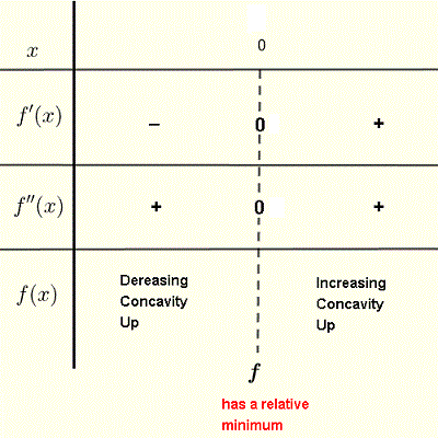
\( f'(x) \) est négative sur \( (-\infty, 0) \), donc \( f \) y est décroissante (Théorème 4.b). \( f'(x) \) est positive sur \( (0, +\infty) \), donc \( f \) y est croissante (Théorème 4.a). D'après le Théorème 2, \( f \) possède un minimum en \( x = 0 \).
Étape 2 : Trouvez la seconde dérivée, son signe et les informations sur la concavité.
\[ f''(x) = 2 \quad (\text{toujours positive}) \]Cela confirme un minimum en \( x = 0 \) puisque \( f''(0) = 2 > 0 \). Le graphique est concave vers le haut sur \( (-\infty, +\infty) \) (Théorème 5.a).
Étape 3 : Trouvez les intersections et les extrema.
Intersection avec l'axe \( y \) : \( f(0) = 0 \). Intersections avec l'axe \( x \) : \( x^2 = 0 \implies x = 0 \).
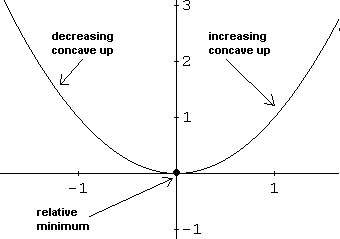
Le point minimum se trouve en \( (0, 0) \).
Étape 4 : Tracez le graphique.
Lorsque \( x \to \pm\infty \), \( f(x) = x^2 \to +\infty \).
Exemple 2
Utilisez les théorèmes des première et seconde dérivées pour tracer la fonction \( f \) définie par :
\[ f(x) = x^3 - 4x^2 + 4x \]Afficher la solution de l'exemple 2
Étape 1 : Première dérivée et points stationnaires.
\[ f'(x) = 3x^2 - 8x + 4 \]La résolution de \( 3x^2 - 8x + 4 = 0 \) donne les points critiques \( x = 2 \) et \( x = \dfrac{2}{3} \).
Étape 2 : Seconde dérivée et points d'inflexion.
\[ f''(x) = 6x - 8 \]La résolution de \( 6x - 8 = 0 \) donne \( x = \dfrac{4}{3} \), où la concavité change (point d'inflexion).
Étape 3 : Intersections et comportement aux limites.
Intersection avec l'axe \( y \) : \( f(0) = 0 \).
Intersections avec l'axe \( x \) : factorisons \( x(x^2 - 4x + 4) = x(x - 2)^2 = 0 \), ce qui donne \( x = 0 \) et \( x = 2 \) (de multiplicité 2).
Lorsque \( x \to +\infty \), \( f(x) \to +\infty \). Lorsque \( x \to -\infty \), \( f(x) \to -\infty \).
Étape 4 : Tableau de signes et graphique.

