Que sont les moindres carrés linéaires ?
Soit \( (x_1, y_1), (x_2, y_2), \dots, (x_N, y_N) \) des points de données expérimentales tels que représentés dans le nuage de points ci-dessous, et supposons que nous souhaitions prédire la variable dépendante \( y \) pour différentes valeurs de la variable indépendante \( x \) à l'aide d'un modèle linéaire de la forme :
\[ y = ax + b \]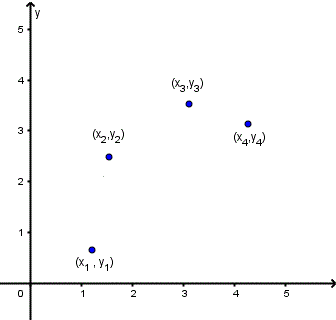
Une procédure très utilisée en mathématiques consiste à minimiser la somme \( D \) des carrés des distances verticales \( d_1, d_2, \dots \) entre le modèle mathématique \( y = f(x) \) et les points expérimentaux, comme illustré dans le graphique ci-dessous.

Dérivation mathématique
Soit \( f(x) = ax + b \) le modèle linéaire à utiliser. Par conséquent, les distances verticales \( d_1, d_2, \dots \) sont données par :
\[ d_1 = |y_1 - (ax_1 + b)|, \quad d_2 = |y_2 - (ax_2 + b)|, \quad \dots \]La somme \( D \) des carrés des distances verticales peut s'écrire :
\[ D = \sum_{i=1}^{N} (y_i - (ax_i + b))^2 \]Les valeurs de \( a \) et \( b \) qui minimisent \( D \) sont celles qui annulent simultanément les dérivées partielles de \( D \) par rapport à \( a \) et \( b \). Par conséquent, nous calculons les dérivées partielles :
\[ \dfrac{\partial D}{\partial a} = \sum_{i=1}^{N} -2x_i(y_i - ax_i - b) \] \[ \dfrac{\partial D}{\partial b} = \sum_{i=1}^{N} -2(y_i - ax_i - b) \]En égalant les deux dérivées à zéro et en divisant par \( -2 \), on obtient le système d'équations normales :
\[ \begin{cases} \sum_{i=1}^{N} x_i(y_i - ax_i - b) = 0 \\ \sum_{i=1}^{N} (y_i - ax_i - b) = 0 \end{cases} \]En développant les sommes :
\[ \begin{cases} \sum_{i=1}^{N} x_iy_i - a \sum_{i=1}^{N} x_i^2 - b \sum_{i=1}^{N} x_i = 0 \\ \sum_{i=1}^{N} y_i - a \sum_{i=1}^{N} x_i - Nb = 0 \end{cases} \]En réarrangeant les termes avec \( a \) et \( b \) à gauche :
\[ \begin{cases} a \sum_{i=1}^{N} x_i^2 + b \sum_{i=1}^{N} x_i = \sum_{i=1}^{N} x_iy_i \\ a \sum_{i=1}^{N} x_i + Nb = \sum_{i=1}^{N} y_i \end{cases} \]Sous forme matricielle :
\[ \begin{bmatrix} \sum_{i=1}^{N} x_i^2 & \sum_{i=1}^{N} x_i \\ \sum_{i=1}^{N} x_i & N \end{bmatrix} \begin{bmatrix} a \\ b \end{bmatrix} = \begin{bmatrix} \sum_{i=1}^{N} x_iy_i \\ \sum_{i=1}^{N} y_i \end{bmatrix} \]À l'aide de la formule de la matrice inverse pour une matrice \( 2 \times 2 \), nous résolvons pour \( a \) et \( b \) :
\[ a = \dfrac{N \sum_{i=1}^{N} x_iy_i - (\sum_{i=1}^{N} x_i)(\sum_{i=1}^{N} y_i)}{N \sum_{i=1}^{N} x_i^2 - (\sum_{i=1}^{N} x_i)^2} \] \[ b = \dfrac{-(\sum_{i=1}^{N} x_i)(\sum_{i=1}^{N} x_iy_i) + (\sum_{i=1}^{N} x_i^2)(\sum_{i=1}^{N} y_i)}{N \sum_{i=1}^{N} x_i^2 - (\sum_{i=1}^{N} x_i)^2} \]Exemple d'application des moindres carrés linéaires
Trouvez l'ajustement par les moindres carrés linéaires \( y = ax + b \) pour les points de données expérimentales donnés par :
\[ \{(1, 2), (3, 4), (2, 6), (4, 8), (5, 12), (6, 13), (7, 15)\} \]Afficher la solution de l'exemple
Établissez un tableau avec les quantités nécessaires :
| \( x_i \) | \( y_i \) | \( x_i y_i \) | \( x_i^2 \) |
|---|---|---|---|
| 1 | 2 | 2 | 1 |
| 3 | 4 | 12 | 9 |
| 2 | 6 | 12 | 4 |
| 4 | 8 | 32 | 16 |
| 5 | 12 | 60 | 25 |
| 6 | 13 | 78 | 36 |
| 7 | 15 | 105 | 49 |
Le nombre total de points est \( N = 7 \).
\( \sum_{i=1}^{7} x_i = 1 + 3 + 2 + 4 + 5 + 6 + 7 = 28 \)
\( \sum_{i=1}^{7} y_i = 2 + 4 + 6 + 8 + 12 + 13 + 15 = 60 \)
\( \sum_{i=1}^{7} x_iy_i = 2 + 12 + 12 + 32 + 60 + 78 + 105 = 301 \)
\( \sum_{i=1}^{7} x_i^2 = 1 + 9 + 4 + 16 + 25 + 36 + 49 = 140 \)
En substituant dans les formules :
\[ a = \dfrac{7 \times 301 - 28 \times 60}{7 \times 140 - 28^2} = \dfrac{2107 - 1680}{980 - 784} = \dfrac{427}{196} \approx 2.1786 \] \[ b = \dfrac{-28 \times 301 + 140 \times 60}{7 \times 140 - 28^2} = \dfrac{-8428 + 8400}{196} = \dfrac{-28}{196} \approx -0.1429 \]Calculateur de moindres carrés linéaires
À partir de points expérimentaux, ce calculateur calcule les coefficients \( a \) et \( b \), l'équation de la droite \( y = ax + b \), ainsi que le coefficient de corrélation. Il trace également les points expérimentaux aux côtés de la droite de meilleur ajustement.
Entrez les points sous la forme \((x_1, y_1), (x_2, y_2), \dots\) séparés par des virgules, ou utilisez l'ensemble de données par défaut.
Survolez le coin supérieur droit du graphique pour télécharger ce dernier au format PNG.
Plus de références et de liens
- Edwards, A. L. An Introduction to Linear Regression and Correlation. San Francisco, CA: W. H. Freeman.
- Dérivées partielles en analyse
- Questions sur la matrice inverse avec solutions
- Tutoriels et problèmes sur les fonctions à plusieurs variables
- Problèmes de régression linéaire avec solutions
- Moindres carrés linéaires sur Wikipédia (en anglais)