Graphing Tangent Functions

Problem: Graph \( f(x) = \tan(x) \) over one period.

Solution:

The function \( \tan x \) is undefined for values of \( x \) equal to \( \frac{\pi}{2} \) and \( -\frac{\pi}{2} \). However, we need to understand the behavior of the graph of \( \tan x \) as \( x \) approaches \( \frac{\pi}{2} \) and \( -\frac{\pi}{2} \).

Let us look at the values of \( \tan x \) for \( x \) close to \( \frac{\pi}{2} \) such that \( x \) is smaller than \( \frac{\pi}{2} \):

We note that as \( x \) approaches \( \frac{\pi}{2} \) from the left (by values smaller than \( \frac{\pi}{2} \)), \( \tan(x) \) increases indefinitely. We say that the graph of \( \tan(x) \) has a vertical asymptote at \( x = \frac{\pi}{2} \). It is represented by a vertical broken red line \( x = \frac{\pi}{2} \) in the graph below.

We now look at the values of \( \tan x \) for \( x \) close to \( -\frac{\pi}{2} \) such that \( x \) is larger than \( -\frac{\pi}{2} \):

We note that as \( x \) approaches \( -\frac{\pi}{2} \) from the right (by values larger than \( -\frac{\pi}{2} \)), \( \tan x \) decreases indefinitely. The graph of \( \tan x \) has a vertical asymptote at \( x = -\frac{\pi}{2} \). It is represented by a vertical broken red line \( x = -\frac{\pi}{2} \) in the graph below.

Using the values above plus \( \tan 0 = 0 \), \( \tan\left(\frac{\pi}{4}\right) = 1 \), and \( \tan\left(-\frac{\pi}{4}\right) = -1 \), we plot the points \( (0, 0) \), \( \left(\frac{\pi}{4}, 1\right) \), and \( \left(-\frac{\pi}{4}, -1\right) \) and the vertical asymptotes:

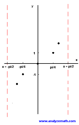
We then draw a smooth curve passing through the points calculated. Close to the vertical asymptotes, the graph either goes upward indefinitely (close to \( x = \frac{\pi}{2} \)) or downward indefinitely (close to \( x = -\frac{\pi}{2} \)):

Summary of graphing \( \tan x \):

• Step 1: Make a table of values over one period:

  \( x \)	\(-\dfrac{\pi}{2}\)	\(-\dfrac{\pi}{4}\)	\(0\)	\(\dfrac{\pi}{4}\)	\(\dfrac{\pi}{2}\)
  \(\tan x\)	VA	\(-1.0\)	\(0.0\)	\(1.0\)	VA

  (where VA means vertical asymptote)
• Step 2: Plot the points and the vertical asymptotes.
• Step 3: Draw a curve passing through all points and rising or falling vertically along the vertical asymptotes.

Problem: Graph function \( f \) given by \( f(x) = 2\tan\left(2x - \dfrac{\pi}{4}\right) \) over one period.

Solution:

Let \( t = 2x - \frac{\pi}{4} \). Let us make a table over one period \( \left(-\frac{\pi}{2}, \frac{\pi}{2}\right) \) using the variable \( t \):

We now use the relationship between \( x \) and \( t \), \( t = 2x - \frac{\pi}{4} \), to find the values of \( x \) corresponding to the values of \( t \). Solving \( t = 2x - \frac{\pi}{4} \) for \( x \) gives: \[ x = \frac{t}{2} + \frac{\pi}{8} \] Adding the \( x \)-row to our table:

Problem: Graph function \( f \) defined by \( f(x) = -\tan\left(x + \dfrac{\pi}{2}\right) \) over one period.

Solution:

Let \( t = x + \frac{\pi}{2} \). We make a table using \( t \) over one period:

Solving \( t = x + \frac{\pi}{2} \) for \( x \) yields \( x = t - \frac{\pi}{2} \). Adding the corresponding \( x \)-values: