Des approches numérique et graphique sont utilisées pour introduire le concept des limites à l'aide d'exemples.
Dans ce qui suit, \( C \) représente la constante d'intégration le cas échéant.
Approche numérique des limites
Exemple 1
Soit \( f(x) = 2x + 2 \) et calculons \( f(x) \) lorsque \( x \) prend des valeurs de plus en plus proches de 1. Nous considérons d'abord des valeurs de \( x \) tendant vers 1 par la gauche (\( x < 1 \)).

Nous considérons maintenant \( x \) s'approchant de 1 par la droite (\( x > 1 \)).
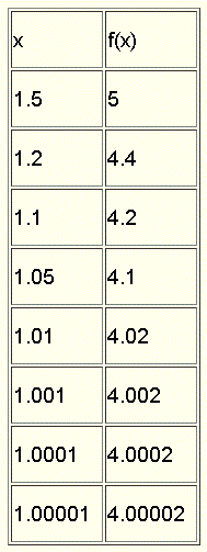
Dans les deux cas, lorsque \( x \) tend vers 1, \( f(x) \) tend vers 4. Intuitivement, nous disons que \( \lim_{x \to 1} f(x) = 4 \).
REMARQUE : Nous parlons des valeurs que prend \( f(x) \) lorsque \( x \) se rapproche de \( 1 \) et non de \( f(1) \). En fait, nous pouvons parler de la limite de \( f(x) \) lorsque \( x \) tend vers \( a \) même lorsque \( f(a) \) n'est pas défini.
Exemple 2
Soit \( g(x) = \dfrac{\sin x}{x} \) et calculons \( g(x) \) lorsque \( x \) prend des valeurs de plus en plus proches de 0. Nous considérons des valeurs de \( x \) s'approchant de 0 par la gauche (\( x < 0 \)) et des valeurs de \( x \) s'approchant de 0 par la droite (\( x > 0 \)).

Ici, nous disons que \( \lim_{x \to 0} g(x) = 1 \). Notez que \( g(0) = \dfrac{\sin 0}{0} = \dfrac{0}{0} \) n'est pas défini en \( x = 0 \).
Approche graphique des limites
Exemple 3
Le graphique ci-dessous montre que lorsque \( x \) tend vers 1 par la gauche, \( y = f(x) \) tend vers 2 et cela peut s'écrire :
\[ \lim_{x \to 1^-} f(x) = 2 \]Lorsque \( x \) tend vers 1 par la droite, \( y = f(x) \) tend vers 4 et cela peut s'écrire :
\[ \lim_{x \to 1^+} f(x) = 4 \]Notez que les limites à gauche et à droite ainsi que \( f(1) = 3 \) sont toutes différentes.

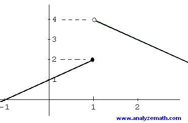
Exemple 4
Ce graphique montre que :
\[ \lim_{x \to 1^-} f(x) = 2 \]Lorsque \( x \) tend vers 1 par la droite, \( y = f(x) \) tend vers 4 et cela peut s'écrire :
\[ \lim_{x \to 1^+} f(x) = 4 \]Notez que la limite à gauche \( \lim_{x \to 1^-} f(x) = 2 \) et \( f(1) = 2 \) sont égales.
Exemple 5
Ce graphique montre que :
\[ \lim_{x \to 0^-} f(x) = 1 \]et
\[ \lim_{x \to 0^+} f(x) = 1 \]Notez que les limites à gauche et à droite sont égales et nous pouvons écrire :
\[ \lim_{x \to 0} f(x) = 1 \]Dans cet exemple, la limite lorsque \( x \) tend vers 0 est égale à \( f(0) = 1 \).

Exemple 6
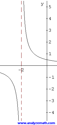
Ce graphique montre que lorsque \( x \) tend vers -2 par la gauche, \( f(x) \) diminue de plus en plus sans borne et il n'y a pas de limite. Nous écrivons :
\[ \lim_{x \to -2^-} f(x) = -\infty \]Lorsque \( x \) tend vers -2 par la droite, \( f(x) \) augmente de plus en plus sans borne et il n'y a pas de limite. Nous écrivons :
\[ \lim_{x \to -2^+} f(x) = +\infty \]Notez que \( -\infty \) et \( +\infty \) sont des symboles et non des nombres. Ce sont des symboles utilisés pour indiquer que la limite n'existe pas.
Exemple 7
Le graphique ci-dessous montre une fonction périodique dont l'ensemble des valeurs est donné par l'intervalle \([-1, 1]\). Si \( x \) augmente sans borne, \( f(x) \) prend des valeurs dans \([-1, 1]\) et n'a pas de limite. Cela peut s'écrire :
\[ \lim_{x \to +\infty} f(x) = \text{n'existe pas} \]Si \( x \) diminue sans borne, \( f(x) \) prend des valeurs dans \([-1, 1]\) et n'a de nouveau pas de limite. Cela peut s'écrire :
\[ \lim_{x \to -\infty} f(x) = \text{n'existe pas} \]

Exemple 8
Si \( x \) augmente sans borne, \( f(x) \) dans le graphique ci-dessous tend vers 2. Cela peut s'écrire :
\[ \lim_{x \to +\infty} f(x) = 2 \]Si \( x \) diminue sans borne, \( f(x) \) tend vers 2. Cela peut s'écrire :
\[ \lim_{x \to -\infty} f(x) = 2 \]
